Optipedia • SPIE Press books opened for your reference.

Explanation of flare from Field Guide to Optical Lithography

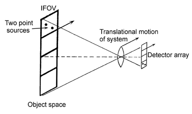
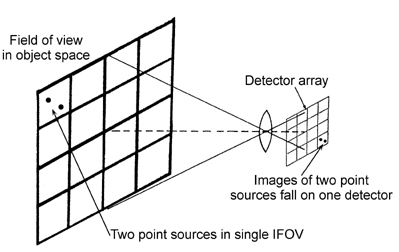
We often think about the object as being imaged onto the detectors, but it is also useful to consider where the detectors are imaged. The footprint of a particular detector, called the instantaneous field of view (IFOV), is the projection of that detector into object space. We consider a scanned imaging system in Fig. 2.1, and a staring focal-plane-array (FPA) imaging system in Fig. 2.2. In each case, the flux falling onto an individual detector produces a single output. Inherent in the finite size of the detector elements is some spatial averaging of the image irradiance. For the configurations shown, we have two closely spaced point sources in the object plane that fall within one detector footprint. The signal output from the sensor will not distinguish the fact that there are two sources. Our first task is to quantify the spatial-frequency filtering inherent in an imaging system with finite-sized detectors.

A square detector of size w × w performs spatial averaging of the scene irradiance that falls on it. When we analyze the situation in one dimension, we find the integration of the scene irradiance f(x) over the detector surface is equivalent to a convolution of f(x) and the rect function¹ that describes the detector responsivity:

By the convolution theorem, Eq. (2.1) is equivalent to filtering in the frequency domain by a transfer function

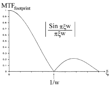
Equation (2.2) shows us that the smaller the sensor photosite dimension is, the broader will be the transfer function. Equation (2.2) is a fundamental MTF component for any imaging system with detectors. In any given situation, the detector footprint may or may not be the main limitation to image quality, but its contribution to a product such as G(ξ,η) = F(ξ,η) x H(ξ,η) is always present. Equation (2.2) is plotted in Fig. (2.3) and we see that the sinc-function MTF has its first zero at ξ = 1/w. It is instructive to consider the following plausibility argument to justify the fact that the footprint MTF = 0 at ξ = 1/w.

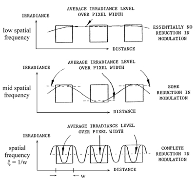
Consider the configuration of Fig. 2.4, representing spatial averaging of an input irradiance waveform by sensors of a given dimension w. The individual sensors may represent either different positions for a scanning sensor or discrete locations in a focal-plane array. We will consider the effect of spatial sampling in a later section. Here we consider exclusively the effect of the finite size of the photosensitive regions of the sensors. We see that at low spatial frequencies there is almost no reduction in modulation of the image irradiance waveform arising from spatial averaging over the surfaces of the photosites. As the spatial frequency increases, the finite size of the detectors becomes more significant. The averaging leads to a decrease in the maximum values and an increase in the minimum values of the image waveform—a decrease in the modulation depth. For the spatial frequency ξ = 1/w, one period of the irradiance waveform just fits onto each detector. Regardless of the position of the input waveform with respect to the photosite boundaries, each sensor will collect exactly the same power (integrated irradiance) level. The MTF is zero at ξ = 1/w because each sensor reads the same level and there is no modulation depth in the resulting output waveform.

Extending our analysis to two dimensions, we consider the simple case of a rectangular detector with different widths along the x and y directions:

By Fourier transformation, we obtain the OTF, which is a two-dimensional sinc function:

and

The impulse response in Eq. (2.3) is separable; that is, h_footprint(x,y) is simply a function of x multiplied by a function of y. The simplicity of the separable case is that both h(x,y) and H(ξ,η) are products of two one-dimensional functions, with the x and y dependences completely separated. Occasionally a situation may arise in which the detector responsivity function is not separable.^2,3 In that case, we can no longer write the MTF as the product of two one-dimensional MTFs. The MTF along the ξ and η spatial frequencies is affected by both x and y profiles of detector footprint. For example, the MTF along the ξ direction is not simply the Fourier transform of the x profile of the footprint but is

Analysis in these situations requires a two-dimensional Fourier transform of the detector footprint. The transfer function can then be evaluated along the ξ or η axis, or along any other desired direction.

References

1. J. Gaskill, Linear Systems, Fourier Transforms, and Optics, Wiley, New York (1978).
2. G. D. Boreman and A. Plogstedt, "Spatial filtering by a nonrectangular detector," Appl. Opt., Vol. 28, p. 1165 (1989).
3. K. J. Barnard and G.D. Boreman, "MTF of hexagonal staring focal plane arrays," Opt. Eng. 30, p. 1915 (1991).