Optipedia • SPIE Press books opened for your reference.
Zernike Polynomials
Excerpt from Field Guide to Interferometric Optical Testing
Zernike polynomials were first derived by Fritz Zernike in 1934. They are useful in expressing wavefront data since they are of the same form as the types 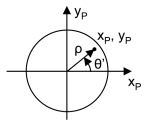 of aberrations often observed in optical tests. These polynomials are a complete set in two variables, ρ and θ', that are orthogonal in a continuous fashion over the unit circle. It is important to note that Zernikes are orthogonal only in a continuous fashion and that in general they will not be orthogonal over a discrete set of data points. Note that θ' is the angle counterclockwise from the xP axis.

There are several common definitions for the Zernike polynomials, so care should be taken that the same set is used when comparing Zernike coefficients. Also note the difference in the definitions of the angle in the measurement plane, θ vs. θ'.
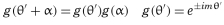
One of the convenient features of Zernike polynomials is that their simple rotational symmetry allows the polynomials to be expressed as products of radial terms and functions of angle, r(ρ)g(θ'), where g(θ') is continuous and repeats itself every 2π radians. The coordinate system can be rotated by an angle a without changing the form of the polynomial. Each Zernike term is referenced by a single number or by two subscripts, n and m, where both are positive integers or zero.
The radial function, r(ρ), must be a polynomial in ρ of degree n and contain no power of ρ less than m. Also, r(ρ) must be even if m is even and odd if m is odd.
| |||||||||||||||||||||||||||||||||||||||||||||||||||||||||||||||||||||||||||||||||||||||||||||||||||||||||||||||||||||||||||||||||||||||||||||||||||||||||||||||||||||||||||||||||||||||||
E. P. Goodwin and J. C. Wyant, Field Guide to Interferometric Optical Testing, SPIE Press, Bellingham, WA (2006).
View SPIE terms of use.

Non-Member: $42.00