Diffraction MTF is a wave-optics calculation for which the only variables (for a given aperture shape) are the aperture diameter D, wavelength λ, and focal length f. The MTFdiffraction is the upper limit to the system’s performance; the effects of optical aberrations are assumed to be negligible. Aberrations increase the spot size and thus contribute to a poorer MTF. The diffraction MTF is based on the overall limiting aperture of the system (the aperture stop). The diffraction effects are only calculated once per system and do not accumulate multiplicatively on an element-by-element basis.
Calculation of diffraction MTF
The diffraction OTF can be calculated as the normalized autocorrelation of the exit pupil of the system. We will show that this is consistent with the definition of Eqs. (1.6), (1.7), and (1.10), which state that the OTF is the Fourier transform of the impulse response. For the incoherent systems we consider, the impulse response h(x,y) is the square of the two-dimensional Fourier transform of the diffracting aperture p(x,y). The magnitude squared of the diffracted electric-field amplitude E in V/cm gives the irradiance profile of the impulse response in W/cm2:

From Eq. (1.23), we must implement a change of variables ξ = x/λf and η = y/λf to express the impulse response (which is a Fourier transform of the pupil function) in terms of image-plane spatial position. We then calculate the diffraction OTF in the usual way, as the Fourier transform of the impulse response h(x,y):

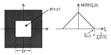
Because of the absolute-value-squared operation, the two transform operations of Eq. (1.24) do not exactly undo each other—the diffraction OTF is the two-dimensional autocorrelation of diffracting aperture p(x,y). The diffraction MTF is thus the magnitude of the (complex) diffraction OTF. As an example of this calculation, we take the simple case of a square aperture, seen in Fig. 1.24:

The autocorrelation of the square is a triangle-shaped function,

with cutoff frequency defined by

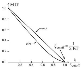
For the case of a circular aperture of diameter D, the system has the same cutoff frequency, ξcutoff = 1/(l F/#), but the MTF has a different functional form:

for ξ < ξcutoff and

for ξ > ξcutoff. These diffraction-limited MTF curves are plotted in Fig. 1.25. The diffraction-limited MTF is an easy-to-calculate upper limit to performance; we need only λ and the F/# to compute it. An optical system cannot perform better than its diffraction-limited MTF—any aberrations will pull the MTF curve down. It is useful to compare the performance specifications of a given system to the diffraction-limited MTF curve to determine the feasibility of the proposed specifications, to decide how much headroom has been left for manufacturing tolerances, or to see what performance is possible within the context of a given choice of λ and F/#.
As an example of the calculations, let us consider the square-aperture system of Fig. 1.26(a) with an object at finite distance. Using the object-space or image-space F/# as appropriate, we can calculate ξcutoff in either the object plane or image plane:

or
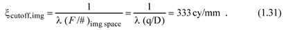
Because p < q, the image is magnified with respect to the object; hence a given feature in the object appears at a lower spatial frequency in the image, so the two frequencies in Eqs. (1.30) and (1.31) represent the same feature. The filtering caused by diffraction from the finite aperture is the same, whether considered in object space or image space. With the cutoff frequency in hand, we can answer questions such as for what image spatial frequency is the MTF 30%? We use Eq. (1.26) to find that 30% MTF is at 70% of the image-plane cutoff frequency, or 223 cy/mm. This calculation is for diffraction-limited performance. Aberrations will narrow the bandwidth of the system, so that the frequency at which the MTF is 30% will be lower than 223 cy/mm.
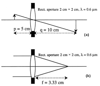
The next example shows the calculation for an object-at-infinity condition, with MTF obtained in object space as well as image space. We obtain the cutoff frequency in the image plane using Eq. (1.27):

As in Fig. 1.26(a), a given feature in Fig. 1.26(b) experiences the same amount of filtering, whether expressed in the image plane or in object space. In the object space, we find the cutoff frequency is

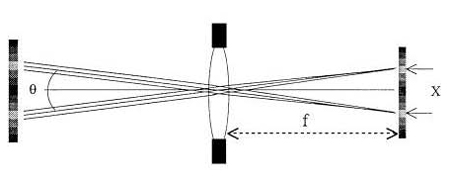
Let us verify that this angular spatial frequency corresponds to the same feature as that in Eq. (1.32). Referring to Fig. 1.27, we use the relationship between object-space angle θ and image-plane distance X,
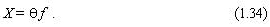
Inverting Eq. (1.34) to obtain the angular spatial frequency 1/θ:
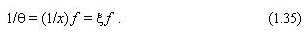
Given that θ is in radians, if X and f have the same units, we can verify the correspondence between the frequencies in Eqs. (1.32) and (1.33):

It is also of interest to verify that the diffraction MTF curves in Fig. 1.25 are consistent with the results of the simple 84% encircled-power diffraction spot-size formula of 2.4 λ (F/#). In Fig. 1.28, we create a one-dimensional spatial frequency with adjacent lines and spaces. We approximate the diffraction spot as having 84% of its flux contained inside a circle of diameter 2.44 λ (F/#), and 16% in a circle of twice the diameter.

The fundamental spatial frequency of the above pattern is

and the modulation depth at this frequency is

in close agreement with Fig. 1.25 for a diffraction-limited circular aperture, at a frequency of ξ = 0.21 ξcutoff .
Reference
- E. Dereniak and G. D. Boreman, Infrared Detectors and Systems, Wiley, New York (1996), referenced figures reprinted by permission of John Wiley and Sons, Inc.
G. D. Boreman, Modulation Transfer Function in Optical and Electro-Optical Systems, SPIE Press, Bellingham, WA (2001).
View SPIE terms of use.